⚖️ Tool for Computing Proximity Scores between Samples
1 2 3 | |
Running SCIMAP 1.3.14
1 2 | |
Quantifying the proximity score with sm.tl.spatial_pscore offers a systematic way to evaluate the closeness between specific cell types as defined by the user.
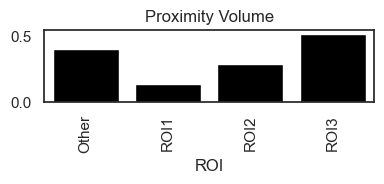
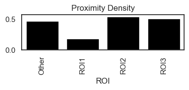
This analysis generates two key metrics: the Proximity Density and the Proximity Volume, both of which are saved in adata.uns.
Proximity Density reflects the ratio of identified interactions to the total number of cells of the interacting types, providing insight into how frequently these cell types interact relative to their population size.
Proximity Volume, on the other hand, compares the number of interactions to the total cell count in the dataset, offering a broader view of the interaction's significance across the entire sample.
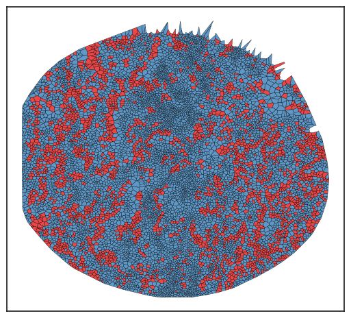
Additionally, the locations of these interaction sites are recorded and saved in adata.obs, allowing for detailed spatial analysis. Running this analysis can elucidate the biological significance of the spatial arrangement of cell types, which is crucial for understanding tissue structure, function, and disease pathology in a more nuanced and quantitative manner.
1 2 3 4 5 6 | |
Identifying neighbours within 50 pixels of every cell
Please check:
adata.obs['spatial_pscore'] &
adata.uns['spatial_pscore'] for results
1 | |
1 | |
As previously noted, the locations of these interactions are recorded, enabling us to spatially plot and examine their distribution within the tissue.
1 2 3 4 5 6 7 8 | |
Save Results
1 2 | |
1 | |