Simple Spatial Analysis
| """
Created on Mon May 16 19:00:32 2022
@author: Ajit Johnson Nirmal
SCIMAP tutorial May 2022
"""
|
| # load packages
import scimap as sm
import scanpy as sc
import pandas as pd
import anndata as ad
|
Tutorial material
You can download the material for this tutorial from the following link:
The jupyter notebook is available here:
| common_path = "/Users/aj/Dropbox (Partners HealthCare)/conferences/scimap_tutorial/may_2022_tutorial/"
#common_path = "C:/Users/ajn16/Dropbox (Partners HealthCare)/conferences/scimap_tutorial/may_2022_tutorial/"
|
| # load data
#adata = sm.pp.mcmicro_to_scimap (image_path= str(common_path) + 'exemplar_001/quantification/unmicst-exemplar-001_cell.csv')
#manual_gate = pd.read_csv(str(common_path) + 'manual_gates.csv')
#adata = sm.pp.rescale (adata, gate=manual_gate)
#phenotype = pd.read_csv(str(common_path) + 'phenotype_workflow.csv')
#adata = sm.tl.phenotype_cells (adata, phenotype=phenotype, label="phenotype")
# add user defined ROI's before proceeding
|
| # load saved anndata object
adata = ad.read(str(common_path) + 'may2022_tutorial.h5ad')
|
Calculate distances between cell types
sm.tl.spatial_distance: The function allows users to calculate the average shortest between phenotypes or clusters of interest (3D data supported).
| adata = sm.tl.spatial_distance (adata,
x_coordinate='X_centroid', y_coordinate='Y_centroid',
z_coordinate=None,
phenotype='phenotype',
subset=None,
imageid='imageid',
label='spatial_distance')
|
Processing Image: unmicst-exemplar-001_cell
| adata.uns['spatial_distance']
|
|
Other Immune cells |
Unknown |
Myeloid |
Tumor |
ASMA+ cells |
Neutrophils |
Treg |
NK cells |
| unmicst-exemplar-001_cell_1 |
0.000000 |
508.809972 |
561.874000 |
547.544519 |
506.115689 |
581.323686 |
570.267087 |
1248.001853 |
| unmicst-exemplar-001_cell_2 |
0.000000 |
25.516388 |
63.601485 |
67.024246 |
27.928445 |
157.289841 |
100.258654 |
816.837582 |
| unmicst-exemplar-001_cell_3 |
0.000000 |
15.315383 |
59.503385 |
56.590105 |
34.479892 |
147.005355 |
96.374952 |
817.307871 |
| unmicst-exemplar-001_cell_4 |
0.000000 |
28.482334 |
13.752853 |
51.500837 |
46.148651 |
111.763900 |
143.243322 |
746.050742 |
| unmicst-exemplar-001_cell_5 |
26.357699 |
0.000000 |
45.589024 |
30.234937 |
58.354288 |
120.715789 |
96.739267 |
824.241184 |
| ... |
... |
... |
... |
... |
... |
... |
... |
... |
| unmicst-exemplar-001_cell_11166 |
0.000000 |
106.320078 |
70.605640 |
96.293073 |
50.637223 |
91.990689 |
43.229554 |
410.740868 |
| unmicst-exemplar-001_cell_11167 |
0.000000 |
31.114913 |
72.531210 |
118.065360 |
54.921505 |
136.323479 |
30.072174 |
399.697389 |
| unmicst-exemplar-001_cell_11168 |
0.000000 |
50.369768 |
70.748013 |
126.968337 |
36.065610 |
123.048957 |
40.094561 |
409.435592 |
| unmicst-exemplar-001_cell_11169 |
0.000000 |
103.275795 |
64.057762 |
91.786425 |
64.741519 |
93.600860 |
35.697321 |
397.194037 |
| unmicst-exemplar-001_cell_11170 |
10.165511 |
0.000000 |
88.288672 |
113.521913 |
86.006117 |
150.562555 |
23.735243 |
389.273701 |
11170 rows × 8 columns
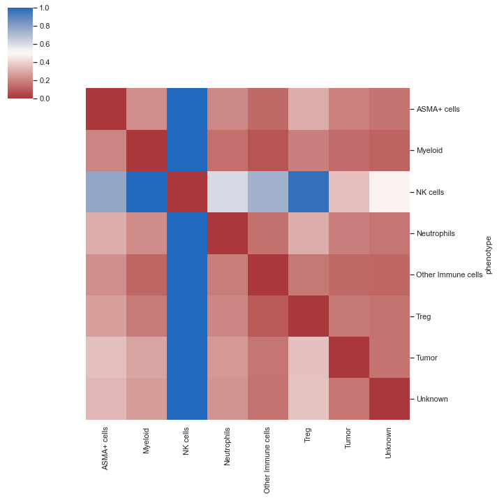
| # summary heatmap
import matplotlib.pyplot as plt
plt.rcParams['figure.figsize'] = [3, 1]
sm.pl.spatial_distance (adata)
|
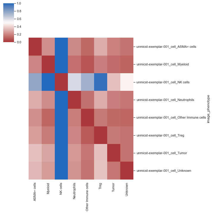
| # Heatmap without summarizing the individual images
sm.pl.spatial_distance (adata, heatmap_summarize=False)
|
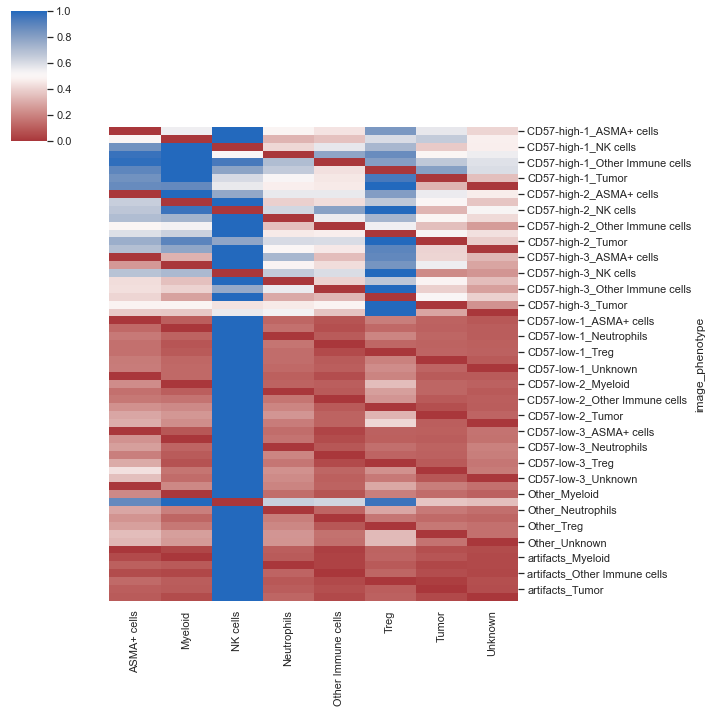
| sm.pl.spatial_distance (adata, heatmap_summarize=False, imageid='ROI_individual')
|
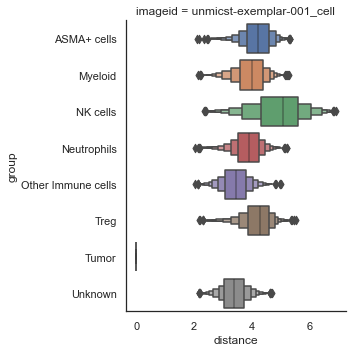
| # Numeric plot of shortest distance of phenotypes
# from tumor cells
sm.pl.spatial_distance (adata, method='numeric',distance_from='Tumor')
|
| sm.pl.spatial_distance (adata, method='numeric',distance_from='Tumor', log=True)
|
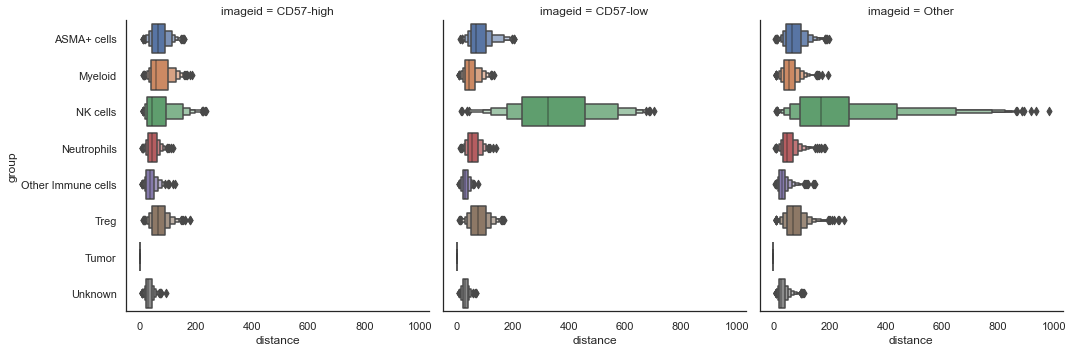
| # plot for each ROI seperately
sm.pl.spatial_distance (adata, method='numeric',distance_from='Tumor', imageid='ROI')
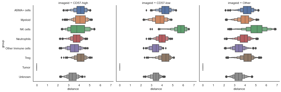
|
| sm.pl.spatial_distance (adata, method='numeric',distance_from='Tumor', imageid='ROI', log=True)
|
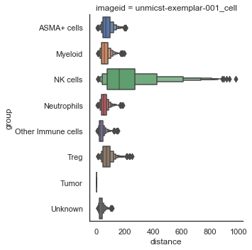
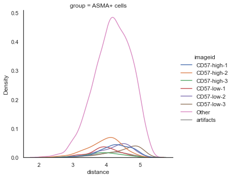
| # Distribution plot of shortest distance of phenotypes from Tumor cells
sm.pl.spatial_distance (adata, method='distribution',distance_from='Tumor',distance_to = 'ASMA+ cells',
imageid='ROI_individual', log=True)
|
Spatial co-occurance analysis
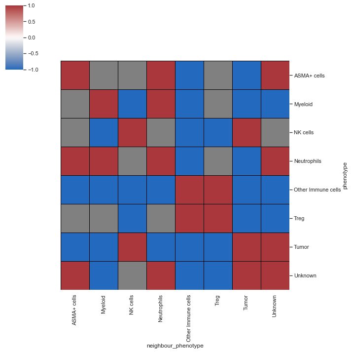
sm.tl.spatial_interaction: The function allows users to computes how likely celltypes are found next to each another compared to random background (3D data supported).
| # Using the radius method to identify local neighbours compute P-values
adata = sm.tl.spatial_interaction (adata,
method='radius',
radius=30,
label='spatial_interaction_radius')
|
Processing Image: ['unmicst-exemplar-001_cell']
Categories (1, object): ['unmicst-exemplar-001_cell']
Identifying neighbours within 30 pixels of every cell
Mapping phenotype to neighbors
Performing 1000 permutations
Consolidating the permutation results
| # Using the KNN method to identify local neighbours
adata = sm.tl.spatial_interaction(adata,
method='knn',
knn=10,
label='spatial_interaction_knn')
|
Processing Image: ['unmicst-exemplar-001_cell']
Categories (1, object): ['unmicst-exemplar-001_cell']
Identifying the 10 nearest neighbours for every cell
Mapping phenotype to neighbors
Performing 1000 permutations
Consolidating the permutation results
| # view results
# spatial_interaction heatmap for a single image
sm.pl.spatial_interaction(adata,
summarize_plot=True,
binary_view=True,
spatial_interaction='spatial_interaction_radius',
row_cluster=False, linewidths=0.75, linecolor='black')
|
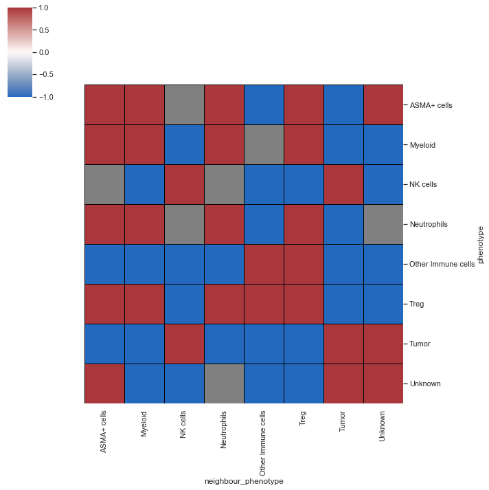
| # spatial_interaction heatmap for a single image
sm.pl.spatial_interaction(adata,
summarize_plot=True,
binary_view=True,
spatial_interaction='spatial_interaction_knn',
row_cluster=False, linewidths=0.75, linecolor='black')
|
| # Pass the ROI's as different images
adata = sm.tl.spatial_interaction(adata,
method='radius',
imageid = 'ROI_individual',
radius=30,
label='spatial_interaction_radius_roi')
|
Processing Image: ['Other']
Categories (1, object): ['Other']
Identifying neighbours within 30 pixels of every cell
Mapping phenotype to neighbors
Performing 1000 permutations
Consolidating the permutation results
Processing Image: ['artifacts']
Categories (1, object): ['artifacts']
Identifying neighbours within 30 pixels of every cell
Mapping phenotype to neighbors
Performing 1000 permutations
Consolidating the permutation results
Processing Image: ['CD57-low-1']
Categories (1, object): ['CD57-low-1']
Identifying neighbours within 30 pixels of every cell
Mapping phenotype to neighbors
Performing 1000 permutations
Consolidating the permutation results
Processing Image: ['CD57-low-3']
Categories (1, object): ['CD57-low-3']
Identifying neighbours within 30 pixels of every cell
Mapping phenotype to neighbors
Performing 1000 permutations
Consolidating the permutation results
Processing Image: ['CD57-low-2']
Categories (1, object): ['CD57-low-2']
Identifying neighbours within 30 pixels of every cell
Mapping phenotype to neighbors
Performing 1000 permutations
Consolidating the permutation results
Processing Image: ['CD57-high-3']
Categories (1, object): ['CD57-high-3']
Identifying neighbours within 30 pixels of every cell
Mapping phenotype to neighbors
Performing 1000 permutations
Consolidating the permutation results
Processing Image: ['CD57-high-1']
Categories (1, object): ['CD57-high-1']
Identifying neighbours within 30 pixels of every cell
Mapping phenotype to neighbors
Performing 1000 permutations
Consolidating the permutation results
Processing Image: ['CD57-high-2']
Categories (1, object): ['CD57-high-2']
Identifying neighbours within 30 pixels of every cell
Mapping phenotype to neighbors
Performing 1000 permutations
Consolidating the permutation results
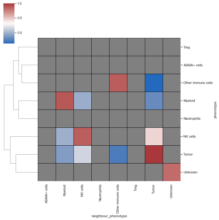
| # spatial_interaction heatmap
sm.pl.spatial_interaction(adata,
summarize_plot=True,
spatial_interaction='spatial_interaction_radius_roi',
row_cluster=True, linewidths=0.75, linecolor='black')
|
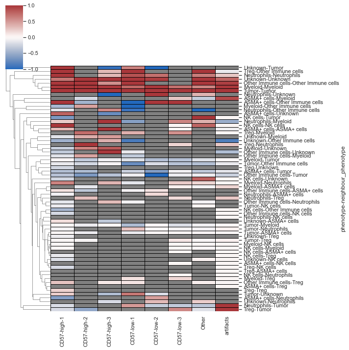
| # spatial_interaction heatmap
sm.pl.spatial_interaction(adata,
summarize_plot=False,
spatial_interaction='spatial_interaction_radius_roi',
yticklabels=True,
row_cluster=True, linewidths=0.75, linecolor='black')
|
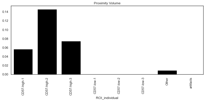
Quantifying the proximity score
sm.tl.spatial_pscore: A scoring system to evaluate user defined proximity between cell types.
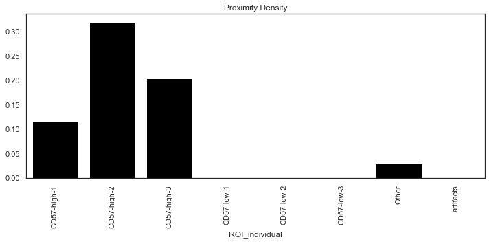
The function generates two scores and saved at adata.uns:
- Proximity Density: Total number of interactions identified divided by the total number of cells of the cell-types that were used for interaction analysis.
- Proximity Volume: Total number of interactions identified divided by the total number of all cells in the data.
The interaction sites are also recorded and saved in adata.obs
| # Calculate the score for proximity between `Tumor CD30+` cells and `M2 Macrophages`
adata = sm.tl.spatial_pscore (adata,proximity= ['Tumor', 'NK cells'],
score_by = 'ROI_individual',
phenotype='phenotype',
method='radius',
radius=20,
subset=None,
label='spatial_pscore')
|
Identifying neighbours within 20 pixels of every cell
Finding neighbourhoods with Tumor
Finding neighbourhoods with NK cells
Please check:
adata.obs['spatial_pscore'] &
adata.uns['spatial_pscore'] for results
| # Plot only `Proximity Volume` scores
plt.figure(figsize=(10, 5))
sm.pl.spatial_pscore (adata, color='Black', plot_score='Proximity Volume')
|
/opt/anaconda3/envs/scimap/lib/python3.9/site-packages/seaborn/_decorators.py:36: FutureWarning:

Pass the following variables as keyword args: x, y. From version 0.12, the only valid positional argument will be `data`, and passing other arguments without an explicit keyword will result in an error or misinterpretation.
| # Plot only `Proximity Density` scores
plt.figure(figsize=(10, 5))
sm.pl.spatial_pscore (adata, color='Black', plot_score='Proximity Density')
|
/opt/anaconda3/envs/scimap/lib/python3.9/site-packages/seaborn/_decorators.py:36: FutureWarning:

Pass the following variables as keyword args: x, y. From version 0.12, the only valid positional argument will be `data`, and passing other arguments without an explicit keyword will result in an error or misinterpretation.
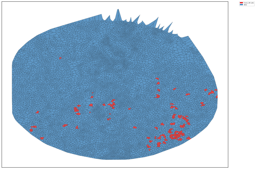
| # voronoi plot
plt.rcParams['figure.figsize'] = [15, 10]
sm.pl.voronoi(adata, color_by='spatial_pscore',
voronoi_edge_color = 'black',
voronoi_line_width = 0.3,
voronoi_alpha = 0.8,
size_max=5000,
overlay_points=None,
plot_legend=True,
legend_size=6)
|
| # save adata
adata.write(str(common_path) + 'may2022_tutorial.h5ad')
|
/opt/anaconda3/envs/scimap/lib/python3.9/site-packages/anndata/_core/anndata.py:1228: FutureWarning:

The `inplace` parameter in pandas.Categorical.reorder_categories is deprecated and will be removed in a future version. Reordering categories will always return a new Categorical object.

... storing 'spatial_pscore' as categorical
This concludes this tutorial